Mapping Inequality in Baltimore¶

Contributers : Sarah Agarrat and Richard Marciano

Introduction¶

After the 1929 Stock Market Crash, thousands of Americans were in danger of home foreclosure. To address this problem and stabilize the market, The Home Owners Loan Coperation (HOLC) was created under the Rooselvelt Administration to asses credibility of families in order to decide to refinance their homes.

The HOLC created area descriptions and maps to "grade" neighborhoods based on racial/ethnic presence, the income of the residents, and environmental factors to determine their "financial risk". A grade of an 'A' (red) , was given to an area characterized as undesirable due to detrimental influences and unfavorable infiltration. Grade 'B' (yellow) areas were characterized by infiltration of a "lower grade population", "lacking homogeniety", and age of the neighborhoods, grade 'C' (blue) areas were completely developed, and 'grade 'D' (green) areas were characterized as "hot spots" that weren't fully built up yet and contained homogeinety. This is called redlining, denying financial services based on race/ethnic background.

Learn more the Mapping Inequality Project here.

This notebook demonstrates computational techniques using attributes from the HOLC Baltimore records. The topics covered are:

Aquiring Data
Data Cleaning and Data Preperation
Data Manipulation
Exploratory Data Analysis and Visualization

Aquiring Data¶

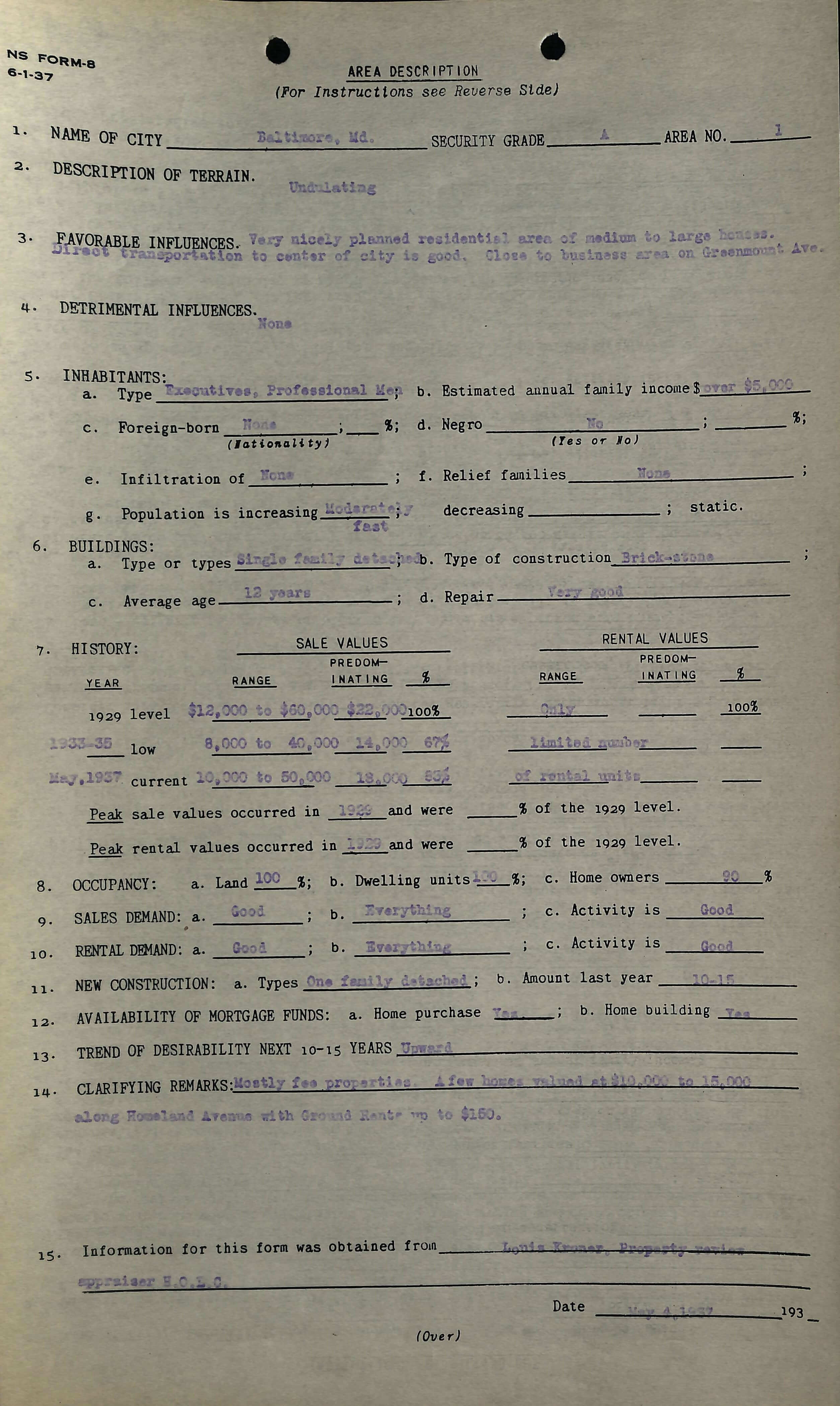
The fields of each record are characteristics of a graded section indicated by the security grade map seen above. These fields have been transcribed and stored in a comma separated value (csv) format.

Using the pandas library, we can create a data frame from the csv. A data frame is a table where every row represents a single unique object, called an entity, and every column represents characteristics of these objects, called attributes.

Importing the Data and Creating a Data Frame¶

In [675]:

# loads the pandas library 
import pandas as pd

# creates data frame named df by reading in the Baltimore csv
df = pd.read_csv("AD_Data_BaltimoreProject.csv")
df.head(n=3)

Out[675]:

	Form	State	City	Security_Grade	Area_Number	Terrain_Description	Favorable_Influences	Detrimental_Influences	INHABITANTS_Type	INHABITANTS_Annual_Income	...	INHABITANTS_Population_Increase	INHABITANTS_Population_Decrease	INHABITANTS_Population_Static	BUILDINGS_Types	BUILDINGS_Construction	BUILDINGS_Age	BUILDINGS_Repair	Ten_Fifteen_Desirability	Remarks	Date
0	NS FORM-8 6-1-37	Maryland	Baltimore	A	2	Rolling	Fairly new suburban area of homogeneous charac...	None	Substantial Middle Class	$3000 - 5,000	...	Fast	NaN	NaN	Detached an row houses	Brick and frame	1 to 10 years	Good	Upward	A recent development with much room for expans...	May 4,1937
1	NS FORM-8 6-1-37	Maryland	Baltimore	A	1	Undulating	Very nicely planned residential area of medium...	None	Executives, Professional Men	over $5000	...	Moderately Fast	NaN	NaN	Single family detached	Brick and Stone	12 years	Very good	Upward	Mostly fee properties. A few homes valued at $...	May 4,1937
2	NS FORM-8 6-1-37	Maryland	Baltimore	A	3	Rolling	Good residential area. Well planned.	Distance to City	Executives, Professional Men	3500 - 7000	...	Moderately Fast	NaN	NaN	One family detached	Brick, Stone, and Frame	1 to 20 years	Good to excellent	Upward	Principally fee property. This section lies in...	May 4,1937

3 rows × 26 columns

In this form, SECUIRITY GRADE has value A and AREA NO. has value 2. This form is located in the first row with index 0 in the data frame.

Data Cleaning and Preparation¶

After obtaining our data, we need to clean it to prepare for data analysis. This includes handling similiar text values and making sure a column of interest contains a single attribute.

Handling Text Values with Similar Meanings¶

The INHABITANTS_Foreignborn varaible indicates whether there are foreigners in a neighborhood section. Observe that different forms used 'No' or 'None' to indicate there are no foreigners and 'Small' , 'Very few' , and 'Mixture' are various ways of indicating there were foreigners. NaN indicates the value in the form is missing.

In [676]:

# selects rows with indices between 0 to 15 included of the 'INHABITANTS_Foreignborn' column
df.ix[0:15,'INHABITANTS_Foreignborn']

Out[676]:

0           No
1         None
2         None
3         None
4         None
5          NaN
6           No
7           No
8           No
9        Small
10    Very few
11          No
12          No
13          No
14          No
15     Mixture
Name: INHABITANTS_Foreignborn, dtype: object

Since columns with categorized values are easier to analyze, we are going to transform this column to indicate whether there are foreigners or not. In Python, None is a special keyword that indicates the cell has a null value. Therefore, we will alter all the 'None' values to 'No' and every other value that indicates there are to 'Yes'.

In [677]:

# replaces the values of 'None' with 'No'
df['INHABITANTS_Foreignborn'] = df['INHABITANTS_Foreignborn'].replace('None', 'No')

# replaces all other values with 'Yes'
for value in df['INHABITANTS_Foreignborn']:
    if value != 'No' and value != 'NaN':
        df['INHABITANTS_Foreignborn'] = df['INHABITANTS_Foreignborn'].replace(value, 'Yes')

df.ix[0:15,'INHABITANTS_Foreignborn']

Out[677]:

0      No
1      No
2      No
3      No
4      No
5     Yes
6      No
7      No
8      No
9     Yes
10    Yes
11     No
12     No
13     No
14     No
15    Yes
Name: INHABITANTS_Foreignborn, dtype: object

Detrimental_Influences are descriptions of a region's undesiriable characteristics. Notice in this case that there are multiple variations of the meaning of 'No' to be replaced.

In [678]:

df.ix[0:15,'Detrimental_Influences']

Out[678]:

0                                          None
1                                          None
2                              Distance to City
3                                          None
4                                          None
5                                           NaN
6                                           No.
7                                          None
8     Few streets of property in poor condition
9                                          None
10                                         None
11                      Built on filled ground.
12                                         None
13                                         None
14                   Distance to center of city
15                                         None
Name: Detrimental_Influences, dtype: object

To handle the multiple words to be replaced we can use an array, a list that holds a fixed number of values of the same type, to store several strings. Then we can replace each occurence in Detrimental_Influences by iterating through the array and using the replace() function.

In [679]:

# declares an array called 'no_words' containing strings that all mean 'No'
no_words = ['No.','no', 'none', 'None']

# interates through no_words and replaces each occurence in Detrimental_Influences
for word in no_words:
    df['Detrimental_Influences'] = df['Detrimental_Influences'].replace( word , 'No')

In [680]:

df.ix[0:15,'Detrimental_Influences']

Out[680]:

0                                            No
1                                            No
2                              Distance to City
3                                            No
4                                            No
5                                           NaN
6                                            No
7                                            No
8     Few streets of property in poor condition
9                                            No
10                                           No
11                      Built on filled ground.
12                                           No
13                                           No
14                   Distance to center of city
15                                           No
Name: Detrimental_Influences, dtype: object

We need to do these same operations for INHABITANTS_Negro, whether residents are African American, and INHABITANTS_Infiltration, which refers to if the area is being infiltrated. Functions are procedures that perform specific tasks. In Python, we can create our own functions or used built-in functions such as replace(). Parameters are variables that are defined in the function definition. Arguments are the values passed into a function.

The replace_values function has three parmeters : attribute, new_word, and words_to_replace.

In [681]:

# this function iterates through an array of words to be replaced and replaces each occurence in the attribute 
# with the new word
def replace_values(attribute, new_word, words_to_replace):
    for word in words_to_replace:
        df[attribute] = df[attribute].replace(word, new_word) 


replace_values('INHABITANTS_Negro', 'No', no_words)
replace_values('INHABITANTS_Infiltration', 'No', no_words)

In [682]:

df.ix[0:15,'INHABITANTS_Infiltration']

Out[682]:

0                  No
1                  No
2                  No
3                  No
4                  No
5                 NaN
6                  No
7                  No
8                  No
9                 NaN
10                 No
11                 No
12                 No
13                 No
14                 No
15    People from C-1
Name: INHABITANTS_Infiltration, dtype: object

Note that we do the same procedure for words meaning 'few', however we could have made these columns have two categories, 'yes' or 'no', and indicate in our data analysis the alterations to our data.

In [683]:

# Various words meaning small 
small_words = ['Nominal','nominal', 'Small','small','Minimum', 'minimum','minimal', 'Very few']

replace_values('INHABITANTS_Negro', 'Few', small_words)
replace_values('INHABITANTS_Infiltration', 'Few', small_words)

In [684]:

df.ix[0:15,'INHABITANTS_Infiltration']

Out[684]:

0                  No
1                  No
2                  No
3                  No
4                  No
5                 NaN
6                  No
7                  No
8                  No
9                 NaN
10                 No
11                 No
12                 No
13                 No
14                 No
15    People from C-1
Name: INHABITANTS_Infiltration, dtype: object

In [685]:

df.ix[0:15,'INHABITANTS_Negro']

Out[685]:

0      No
1      No
2      No
3      No
4      No
5     NaN
6      No
7      No
8      No
9      No
10     No
11     No
12     No
13     No
14     No
15     No
Name: INHABITANTS_Negro, dtype: object

We can clean up the values of INHABITANTS_Population_Increase, how the population is increasing in an area, by choosing standard categories for the rate the population.

In [686]:

 df.ix[0:15,'INHABITANTS_Population_Increase']

Out[686]:

0               Fast 
1     Moderately Fast
2     Moderately Fast
3              Slowly
4     Moderately Fast
5                 NaN
6                 NaN
7              Slowly
8     Moderately Fast
9     Moderately Fast
10                NaN
11             Slowly
12             Slowly
13         Moderately
14             Slowly
15              Fast 
Name: INHABITANTS_Population_Increase, dtype: object

We will define rates of the population as very slowly, slowly, moderately, moderately fast, fast based on the data.

In [687]:

# defines values to replace in the table 
very_slowly = ['Very Slowly', 'very slowly', 'very Slowly']
slowly = ['slowly', 'fairly slowly']
moderately = ['moderately']
moderately_fast = ['Moderately Fast', 'moderately Fast', 'moderately fast']
fast = ['very fast', 'Very Fast', 'fast']

# applies function to obtain our new values 
replace_values('INHABITANTS_Population_Increase', 'Very slowly', very_slowly)
replace_values('INHABITANTS_Population_Increase', 'Slowly', slowly)
replace_values('INHABITANTS_Population_Increase', 'Moderately', moderately )
replace_values('INHABITANTS_Population_Increase', 'Moderately fast', moderately_fast)
replace_values('INHABITANTS_Population_Increase', 'Moderately fast', moderately_fast)
replace_values('INHABITANTS_Population_Increase', 'Fast', fast)

In [688]:

 df.ix[0:15,'INHABITANTS_Population_Increase']

Out[688]:

0               Fast 
1     Moderately fast
2     Moderately fast
3              Slowly
4     Moderately fast
5                 NaN
6                 NaN
7              Slowly
8     Moderately fast
9     Moderately fast
10                NaN
11             Slowly
12             Slowly
13         Moderately
14             Slowly
15              Fast 
Name: INHABITANTS_Population_Increase, dtype: object

String Parsing to Extract Data¶

Some of the cities have corresponding suburbs followed by a dash. We can extract the suburbs and create a new column using str.split().

In [689]:

df.ix[16:30,'City']

Out[689]:

16                                Baltimore 
17                       Baltimore - Dundalk
18                                 Baltimore
19                  Baltimore - Metropolitan
20                                 Baltimore
21                  Baltimore - Metropolitan
22                                 Baltimore
23                   Baltimore - Sub. Burton
24    Baltimore - Sub. Mt. Washington Summit
25                Baltimore - Sub. Villahove
26            Baltimore - Sub. Colonial Park
27        Baltimore - Sub. Linthicum Heights
28                                 Baltimore
29                                 Baltimore
30                                 Baltimore
Name: City, dtype: object

A new data frame seperate is created with two columns seperated based on str.split, where n=1 indicates the string is split once. We create two new attributes in the original data frame, City_clean and Suburb. Then we drop the old City city column and rename our new City attribute.

In [690]:

# creates a new data frame that splits the values in the orginal data frame on the '-' character 
newdf = df["City"].str.split('-', n = 1, expand = True) 
newdf.head()

# creates two new columns 
df['City_clean'] = newdf[0]
df['Suburb'] = newdf[1]

# removes the old column
df.drop(["City"], axis = 1, inplace = True) 

# renames as 'City'
df.rename(index=str, columns={"City_clean": "City"});

In [691]:

df.ix[16:30,['Suburb']]

Out[691]:

	Suburb
16	None
17	Dundalk
18	None
19	Metropolitan
20	None
21	Metropolitan
22	None
23	Sub. Burton
24	Sub. Mt. Washington Summit
25	Sub. Villahove
26	Sub. Colonial Park
27	Sub. Linthicum Heights
28	None
29	None
30	None

The BUILDINGS_Age attribute represents the range of the age of the buildings in a region. Notice the range is given is given as a string of text. For purpose of analysis, we would like to extract the upper end of the range and create a column of numeric values.

In [692]:

df.ix[0:15,'BUILDINGS_Age']

Out[692]:

0      1 to 10 years
1           12 years
2      1 to 20 years
3           10 years
4      1 to 20 years
5                NaN
6           25 years
7     15 to 25 years
8           15 years
9      5 to 25 years
10          20 years
11     5 to 10 years
12          10 years
13          25 years
14     1 to 20 years
15     6 to 25 years
Name: BUILDINGS_Age, dtype: object

Observe that the numeric value at the end of the range is always the last number followed by the string years. We use specific string patterns called regular expressions (regex) and str.extract() to create a new attribute called max_building_age.

In [693]:

df['max_building_age'] = df['BUILDINGS_Age'].str.extract('(\d+)(?!.*\d)', expand=True)

The regular expression in this example is (\d+)(?!.*\d) and was tested using Pythex, a regex editor. We could have imported re , Python's regular expression library, to perform the same task, however this notebook consistenly uses str() functions.

In [694]:

df.ix[0:15,['BUILDINGS_Age','max_building_age']]

Out[694]:

	BUILDINGS_Age	max_building_age
0	1 to 10 years	10
1	12 years	12
2	1 to 20 years	20
3	10 years	10
4	1 to 20 years	20
5	NaN	NaN
6	25 years	25
7	15 to 25 years	25
8	15 years	15
9	5 to 25 years	25
10	20 years	20
11	5 to 10 years	10
12	10 years	10
13	25 years	25
14	1 to 20 years	20
15	6 to 25 years	25

The Date, the date indicated on the form, has three attributes with the pattern given by month day, year. As previously stated, we would like to have a single attribute per column.

In [695]:

df.ix[0:3,['Date']]

Out[695]:

	Date
0	May 4,1937
1	May 4,1937
2	May 4,1937
3	May 4,1937

We can seperate this column into three columns: Month, Day, and Year using str.extract() and regex patterns (\d\d\d\d) to indicate four digit year, (\d) to indicate a single digit day, and [A-Z]\w{0,} to indicate aplhanumeric text to extract the month. Note that regex can also be used to reformat the date column.

In [696]:

# extracts the year 
df['Year'] = df['Date'].str.extract('(\d\d\d\d)', expand=True)

# extracts day  
df['Day'] = df['Date'].str.extract('(\d)', expand=True)

# extracts month 
df['Month'] = df['Date'].str.extract('([A-Z]\w{0,})', expand=True)

df.ix[0:3,['Date','Month','Day','Year']]

Out[696]:

	Date	Month	Day	Year
0	May 4,1937	May	4	1937
1	May 4,1937	May	4	1937
2	May 4,1937	May	4	1937
3	May 4,1937	May	4	1937

Similar to BUILDINGS_Age, INHABITANTS_Annual_Income, the range of income of residents in a section, is a string of text and we would like to extract the numeric value at the end of the range.

In [697]:

df.ix[0:7,['INHABITANTS_Annual_Income']]

Out[697]:

	INHABITANTS_Annual_Income
0	$3000 - 5,000
1	over $5000
2	3500 - 7000
3	over $5000
4	$3,500 - $10,000
5	NaN
6	over $4000
7	over $5000

Observe that some values are located after '$', some inlcude '-', and others include ','.Since the pattern to extract the last numeric value varies, we use str.replace(), str.extract, and regex in a sequence of operations to create a new column max_annual_income.

In [698]:

# replaces anything that is not a digit or ',' with empty space
df['max_annual_income'] = df['INHABITANTS_Annual_Income'].str.replace('[^\d(,)]',' ')

In [699]:

df.ix[0:7,['max_annual_income']]

Out[699]:

	max_annual_income
0	3000 5,000
1	5000
2	3500 7000
3	5000
4	3,500 10,000
5	NaN
6	4000
7	5000

We did not include the delimeter in the previous str.replace() operation because their positions would have been replaced by an empty space. Now we want to remove delimeters.

In [700]:

# removes delimeter by replacing ',' with ''
df['max_annual_income'] = df['max_annual_income'].str.replace('[(,)]','')

In [701]:

df.ix[0:7,['max_annual_income']]

Out[701]:

	max_annual_income
0	3000 5000
1	5000
2	3500 7000
3	5000
4	3500 10000
5	NaN
6	4000
7	5000

Finally, we can extract the last number.

In [702]:

# extracts the second or last number 
df['max_annual_income'] = df['max_annual_income'].str.extract('(\d+)(?!.*\d)', expand=True)

In [703]:

df.ix[0:7,['max_annual_income']]

Out[703]:

	max_annual_income
0	5000
1	5000
2	7000
3	5000
4	10000
5	NaN
6	4000
7	5000

Data Manipulation¶

Some aspects of data manipulation, altering data to make it easier to read or use, include sorting and grouping attributes and encoding categorical variables.

Sorting and Grouping¶

The values of Area_Number are out of order and we want these values to be sorted by Security_Grade.

In [704]:

# removes any additional spaces from Security_Grade
df['Security_Grade'] = df['Security_Grade'].str.replace('[\W]','')
# converts 'Area_Number' from type object to type 'numeric'
df['Area_Number'] = pd.to_numeric(df['Area_Number'])
df.ix[0:10,['Security_Grade','Area_Number']]

Out[704]:

	Security_Grade	Area_Number
0	A	2
1	A	1
2	A	3
3	A	4
4	A	5
5	A	6
6	B	1
7	B	2
8	B	3
9	B	4
10	B	5

To do this, we created use the sort_values() function on the original data frame and reset the index. First, the data is sorted and grouped by Security_Grade and then Area_Number is sorted in increasing order.

In [705]:

df = df.sort_values(by=['Security_Grade', 'Area_Number'])
# resets the index starting from 0
df = df.reset_index(drop=True)
df.ix[0:10,['Security_Grade','Area_Number']]

Out[705]:

	Security_Grade	Area_Number
0	A	1
1	A	2
2	A	3
3	A	4
4	A	5
5	A	6
6	B	1
7	B	2
8	B	3
9	B	4
10	B	5

Encoding Categorical Data¶

In [706]:

 df.ix[0:15,'INHABITANTS_Population_Increase']

Out[706]:

0     Moderately fast
1               Fast 
2     Moderately fast
3              Slowly
4     Moderately fast
5                 NaN
6                 NaN
7              Slowly
8     Moderately fast
9     Moderately fast
10                NaN
11             Slowly
12             Slowly
13         Moderately
14             Slowly
15              Fast 
Name: INHABITANTS_Population_Increase, dtype: object

Exploratory Data Analysis and Visualization¶

The goal of exploratory data analysis (EDA) is to explore attributes across multiple entities to decide what statistical or machine learning techniques to apply to the data. Visualizations are used to assist in understanding the data.

The .describe() function summarizes a data frame column. Since the data type of max_building_age is currently type 'object', which in python is an indcator of type 'string', we have to first convert this attribute into a numeric value.

In [707]:

df['max_building_age'].describe()

Out[707]:

count     46
unique    12
top       25
freq       9
Name: max_building_age, dtype: object

Now that max_building_age is numeric type, we see that describe() provides summary statistics on this attribute.

In [708]:

# converts max_building age to numeric type
df["max_building_age"] = pd.to_numeric(df["max_building_age"])
df['max_building_age'].describe()

Out[708]:

count    46.000000
mean     30.086957
std      16.497577
min      10.000000
25%      20.000000
50%      25.000000
75%      40.000000
max      65.000000
Name: max_building_age, dtype: float64

We can the same operations to max_annual_income.

In [709]:

df['max_annual_income'].describe()

Out[709]:

count       46
unique      12
top       2500
freq         8
Name: max_annual_income, dtype: object

In [710]:

df['max_annual_income'] = pd.to_numeric(df['max_annual_income'])
df['max_annual_income'].describe()

Out[710]:

count       46.000000
mean      3139.130435
std       2009.806874
min       1000.000000
25%       1850.000000
50%       2750.000000
75%       4000.000000
max      10000.000000
Name: max_annual_income, dtype: float64

Finally we create some plots our data. A scatter plot and a bar chart are shown below.

In [734]:

df.plot(kind='scatter',x='max_building_age',y='max_annual_income',color='red', title='max_annual income vs. max_building age')
plt.show()

In [730]:

df.groupby('Security_Grade')['max_annual_income'].nunique().plot(kind='bar', title='Max Annual Income by Security_Grade')
plt.show()

In [731]:

df.groupby('Security_Grade')['max_building_age'].nunique().plot(kind='bar', title='Max Building Age by Security_Grade')
plt.show()