Results
Sample Queries
To explore the data model I created once it was populated with the directory data, I ran two sets of sample queries - the first set was queries I ran in the original assignment, and the second were new queries created for this project.
Old Queries Rerun
The first query I wanted to re-test was one that investigated relationships between a person's marital status and their address and type of dwelling.
#returns marital status, person, dwelling type
MATCH (m:MaritalStatus)-[ms:HasMaritalStatus]-(p:Person)-[la:LivesAt]-(a:Address)-[ia:IsA]-(d:Dwelling)
RETURN m, ms, p, la, a, ia, d
With the new version of the database, the result graph looks something like this:
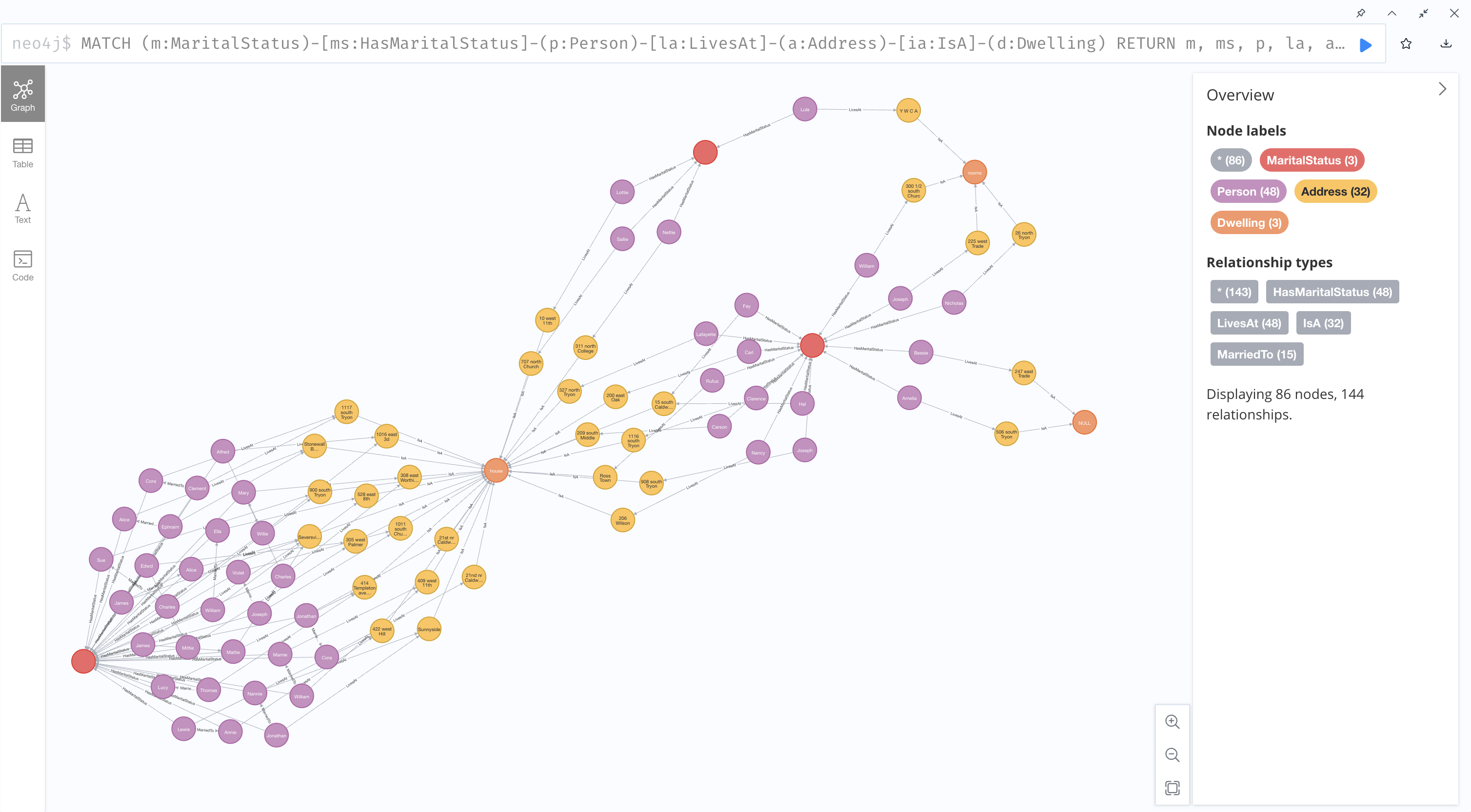
Not only is this graph more spaced out and easier to visually dissect, it also provides a more accurate sense of the number of individuals living in each type of dwelling because spouses appear as distinct nodes.
The second rerun query investigated relationships between marital status and race:
#returns person, marital status, race
MATCH (m:MaritalStatus)-[ms:HasMaritalStatus]-(p:Person)-[hr:HasRace]-(r:Race)
RETURN p, hr, r, m, ms
resulting in the following graph:
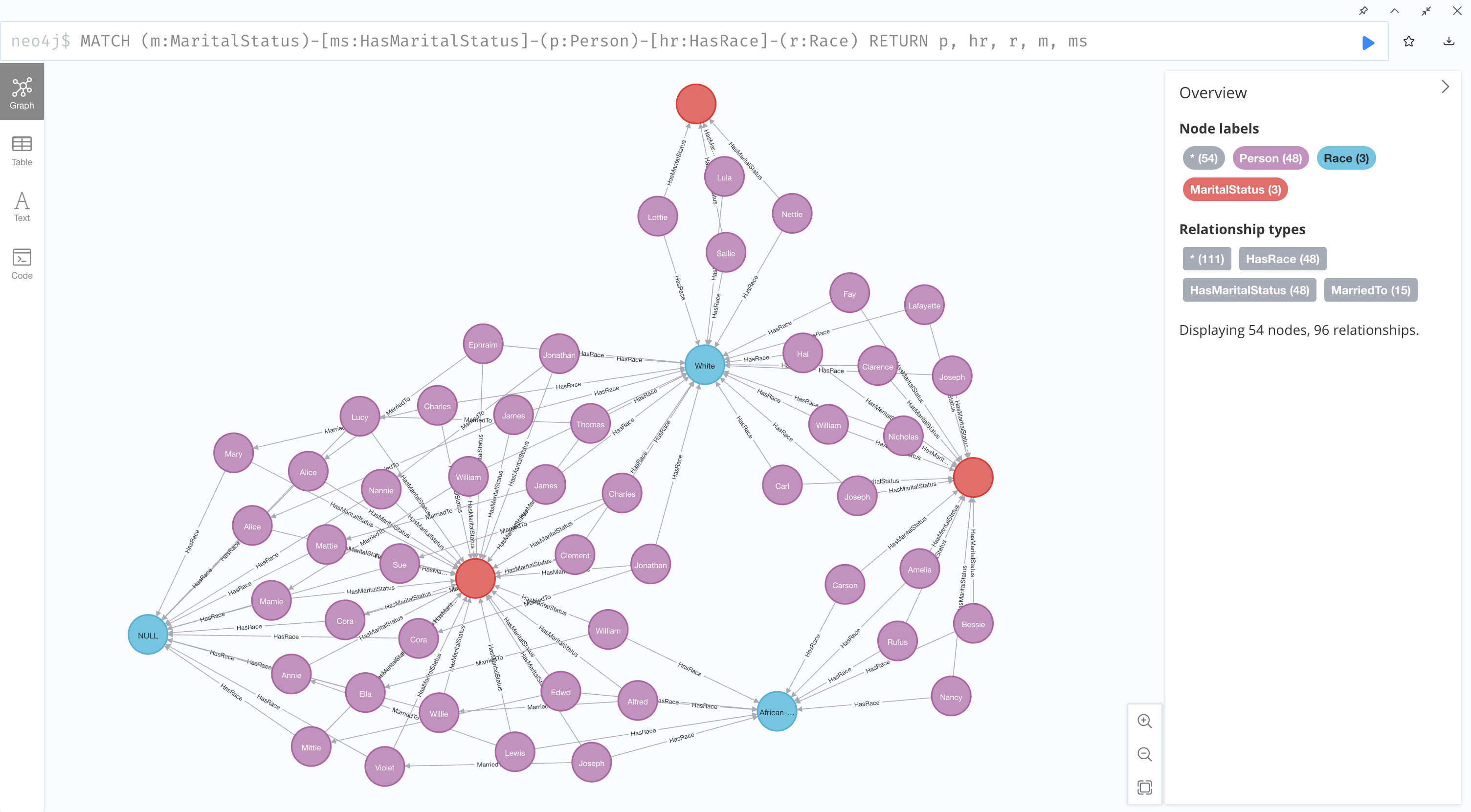
This one didn't have as dramatic of a change, because as previously mentioned, I did not assume the race of any spouses. However, it does still appear more streamlined because the Person nodes are connected to the MaritalStatus nodes, and not combined MaritalStatus/Spouse nodes.
New Queries
The following queries were created specifically to test the capabilities of this data model. While they're not particularly complex, I feel that they do a good job of demonstrating the additional aspects of the dataset that can be accessed through this data model.
#view person to person relationships
MATCH (p1:Person) - [] - (p2: Person)
RETURN p1, p2
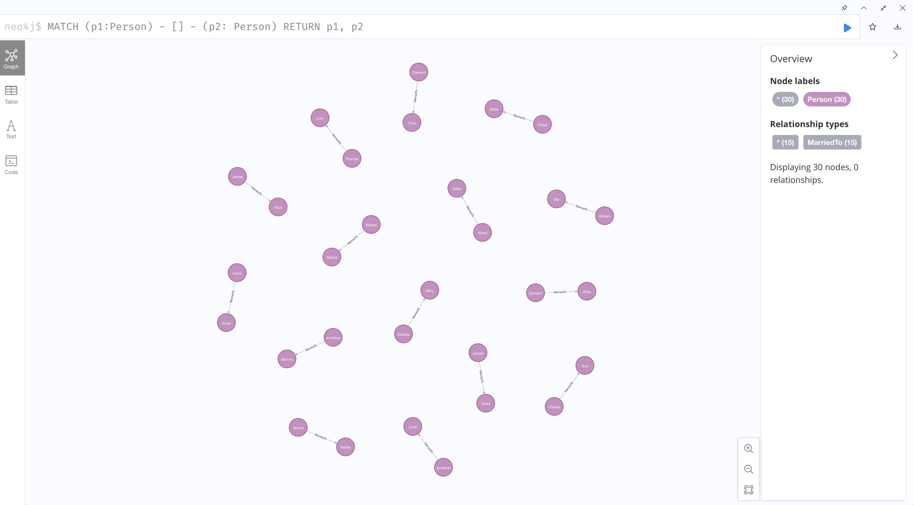
While this result graph isn't particularly exciting, the fact that I was able to generate it at all demonstrates that the data model created for this project works as intended.
#jobs held by married people
MATCH (m:MaritalStatus {MaritalType: 'Married'})-[ms:HasMaritalStatus]-(p:Person)-[hj:HasJob]-(j:Job)
RETURN p, hj, j
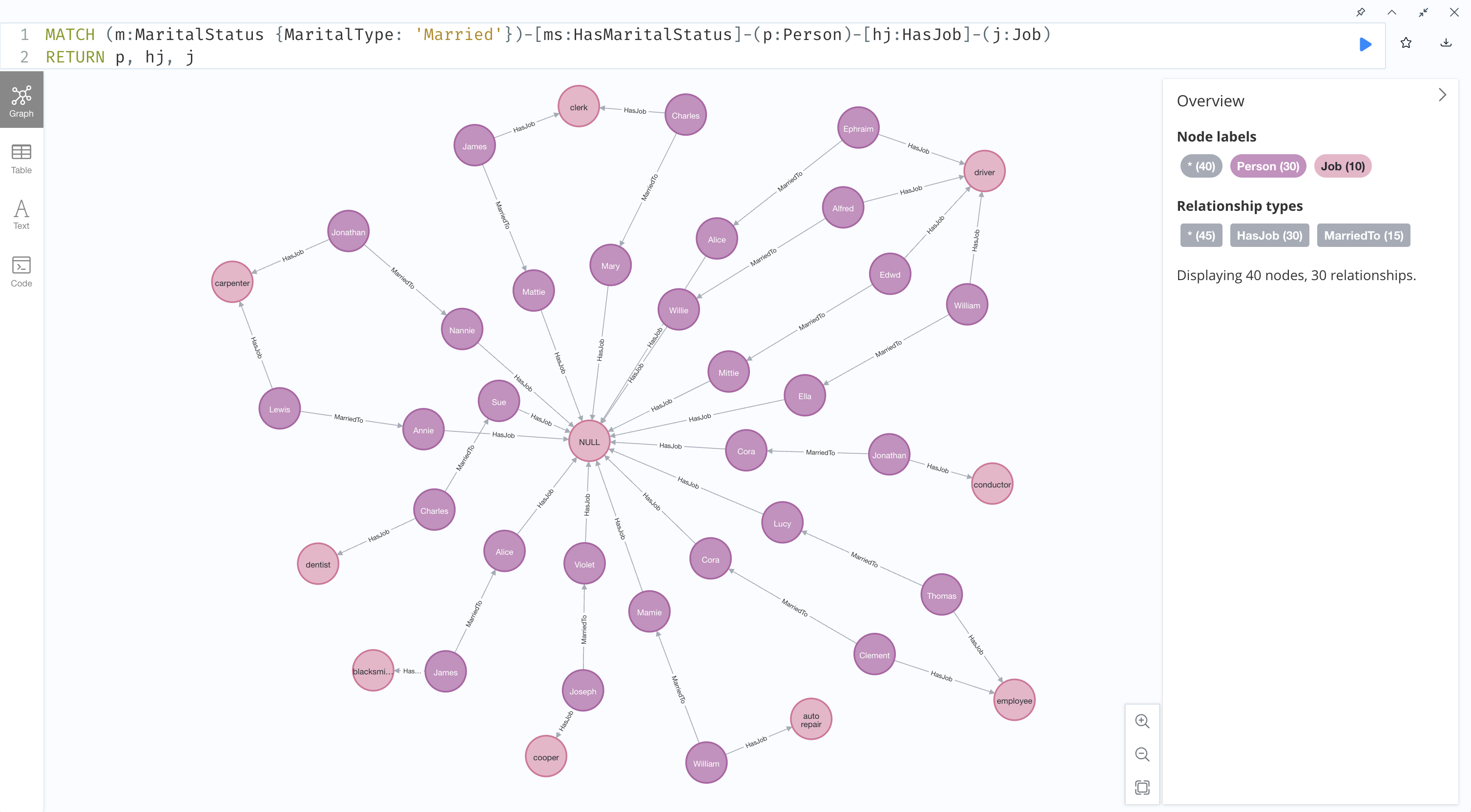
This query produced an interesting result because I chose not to display marital status nodes in the output graph, so we get a ring of unemployed wives in the center surrounded by an outer ring of their husbands and each man's job.
# returns person, address, dwelling type
MATCH (p:Person)-[la:LivesAt]-(a:Address)-[ia:IsA]-(d:Dwelling)
RETURN p, la, a, ia, d
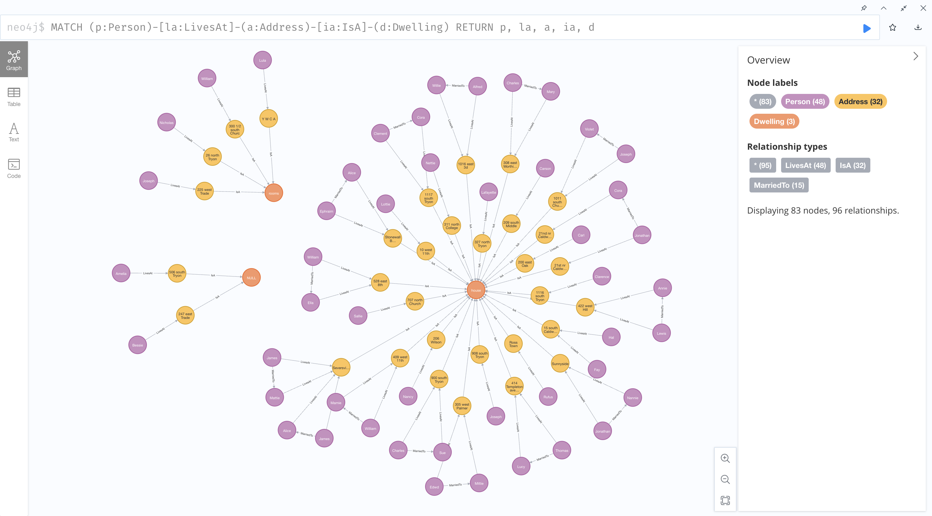
This query is a variation on one from the original assignment that was re-run above, omitting the Marital Status nodes. This provides a relatively tidy depiction of each household unit.
Thoughts on Future Work
Expansion and Scalability
It would certainly be possible to expand this project to encompass larger versions of the data set - either the 160 record set used for the original assignment or the full 16,000 record set. However, scalability may be difficult because the data manipulation had to be done manually in Excel. I was not able to use OpenRefine for this project because the data modifications I was executing involved the creation of a large number of new rows, and OpenRefine is not well suited to that. Given more time it may be possible to find an automated workaround for this issue, but it was not feasible within the time constraints of this iteration of the project.
Opening Up Historical Data
As a proof of concept, this project and its resultant products provide compelling evidence that adjusting data models can open up historical datasets in new ways. Compared to the previously used model, the data model I created allows for queries that drill down deeper into the dataset, separating individual facets in a way that facilitates exploration of the complexities and a more detailed view of the bigger picture. The analytical process applied during the modeling stage of this project could be adapted to fit almost any structured dataset - all that is required is a little flexible thinking.
Return: Project Overview